Payback Is an Operating Result, Not a Machine-Price Ratio
An OCC recycling plant may look financially attractive in a quotation but still fall short of its payback target once production begins. The problem is usually not a single major error, but several small assumptions that all make the project look better than it really is. Nameplate capacity may be counted as saleable output, scheduled hours as productive hours, and every incoming tonne as recovered fiber. Labor may be calculated at the basic wage rate rather than the full employer cost, while the first month of operation is treated as though the line has already reached stable production.
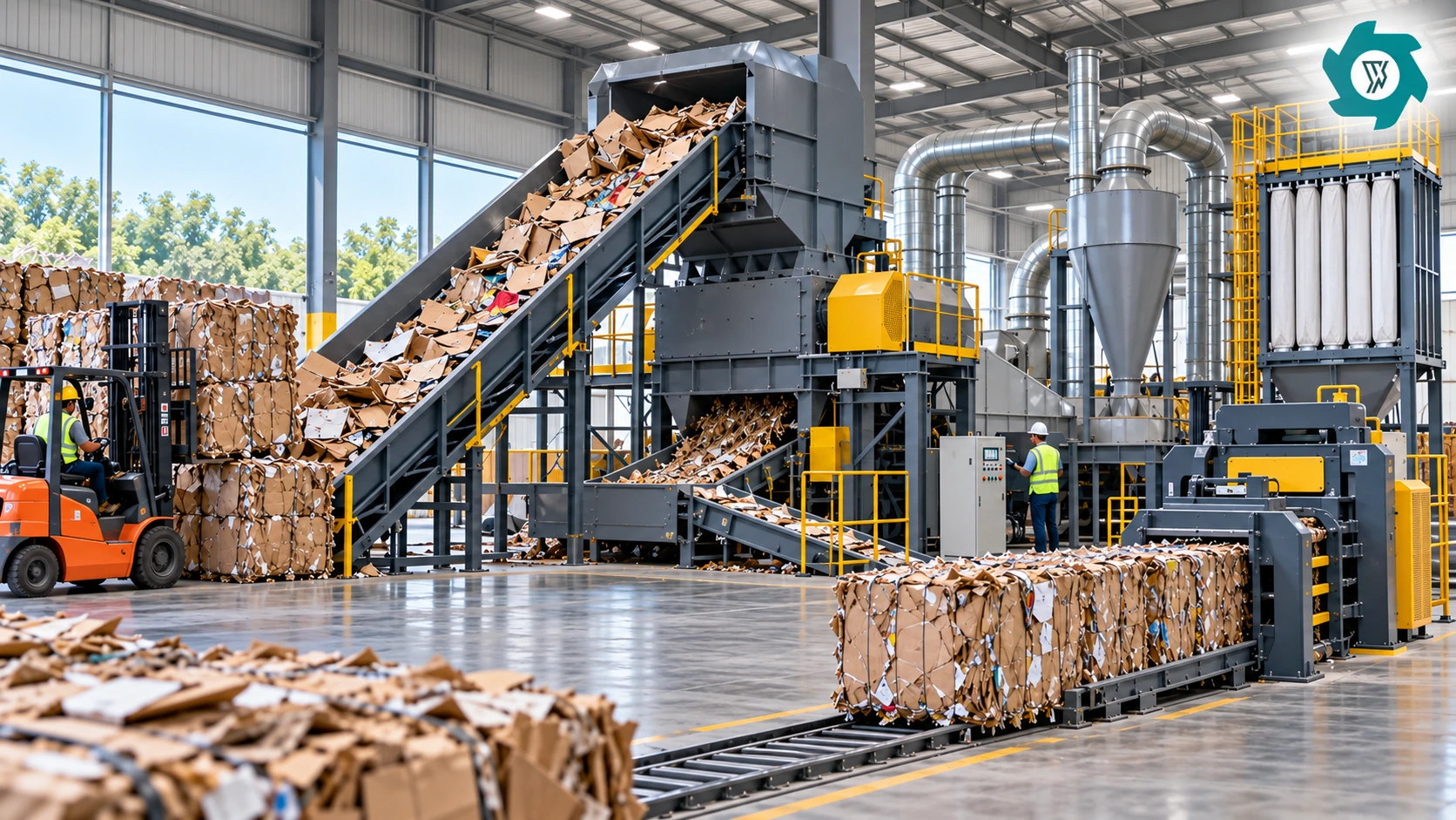
That is why an ROI discussion should start with the physical flow of material and time. A dry OCC line receives real cardboard with moisture, wire, film, dirt and dimensional variation. It then has to meter that feed, reduce and open it, remove defined contaminants, control dust, move the product, handle rejects and keep the back end clear. The plant earns its return only when those functions produce accepted output that can be sold or used downstream. For the process boundary itself, review the OCC recycling plant before building the financial model.
The U.S. recovered-paper market is large, but market size does not guarantee an individual project return. AF&PA reported that more than 33 million tons of cardboard were recycled in the United States in 2025 and estimated the cardboard recycling rate at 70%–75%.[1] A plant still has to win on its own feed cost, output value, reliability and operating discipline.
First Separate ROI, Simple Payback and Life-Cycle Economics
Project teams often use “ROI” and “payback” interchangeably. Simple payback asks how long cumulative cash contribution takes to recover the initial cash investment. A conventional ROI percentage compares a defined gain with a defined investment over a stated period. Net present value and internal rate of return go further by considering the timing of future cash flows.
For early equipment screening, simple payback can be useful because it forces the team to connect investment with annual operating contribution. It should not be mistaken for a complete investment appraisal. U.S. Department of Energy life-cycle cost guidance distinguishes initial cost from recurring operating costs and uses measures including payback, net savings and internal rate of return when comparing long-lived alternatives.[2] Once an OCC project moves from technical screening to final funding approval, the finance team should add tax, financing, depreciation, discount rate and terminal value according to the company’s own rules.
The Five Variables That Usually Move Payback the Most
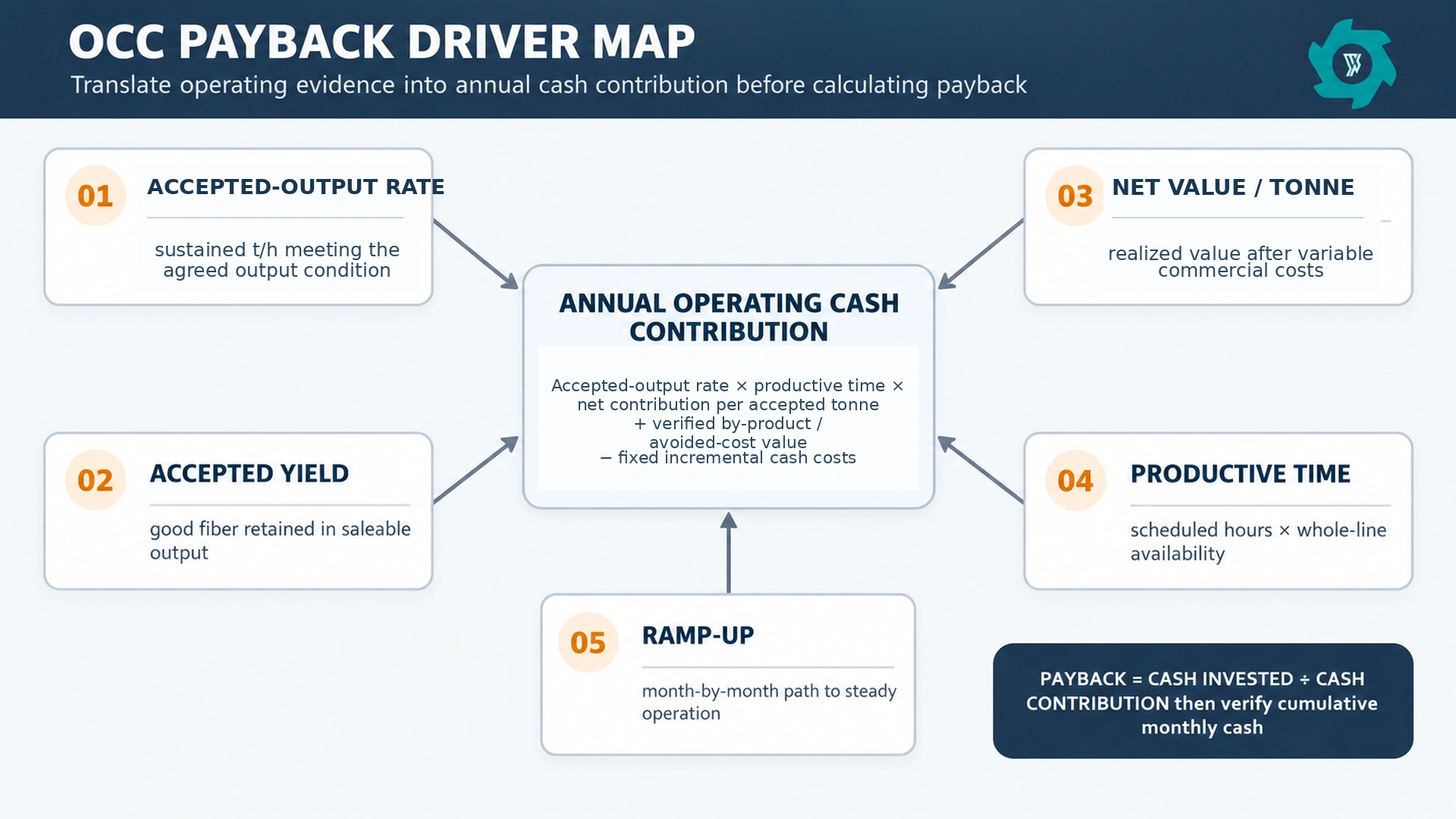
An equipment quotation is visible and easy to compare. The more important ROI variables are often less visible because they sit across operations, purchasing, sales and maintenance. Build the model around five drivers: sustained accepted-output rate during productive running time, accepted yield, net value per accepted ton, operating availability and the ramp-up path to stable production. Energy, labor, wear parts, rejects and working capital then sit under those drivers as explicit cash lines rather than being buried inside a single “operating cost” percentage.
1. Use Accepted Output per Productive Running Hour, Not Nameplate Throughput
The first production input should be the sustained accepted-output rate achieved while the complete line is actually running. Operating availability should then be modeled separately to determine how many productive running hours are available from the scheduled production calendar. Do not start with the maximum feed rate of the shredder. A complete line can be constrained by bale preparation, feed control, mechanical opening, dust discharge, reject bins, a downstream baler or the time required to clear difficult material. The slowest practical interface determines what the business can ship.
This distinction changes the financial model immediately. Suppose a line is scheduled for 2,000 hours per year and achieves 85% operating availability. That leaves 1,700 productive running hours. A spreadsheet using 3.0 t/h nameplate capacity would imply 6,000 theoretical tonnes if availability were ignored. If the complete line instead sustains 2.3 t/h of accepted output during actual running time, annual accepted output is about 3,910 tonnes. The difference is not a minor engineering detail; it may represent a large portion of the expected annual contribution.
Use the acceptance-test definition as the financial definition. Accepted output should meet the agreed physical and quality condition. During testing, record running time and elapsed time, plus stops, reversals, operator interventions, manual clearing, downstream holds and maintenance stops. The detailed test method belongs in the OCC recycling plant RFQ checklist; the ROI model only needs the result translated into an auditable accepted-output rate.
2. Treat Yield as a Commercial Variable, Not Just a Mass-Balance Percentage
Two plants can process the same incoming tonnage and create different financial results because they lose different amounts of usable fiber. Yield should therefore mean accepted output divided by accepted input under a defined test boundary. It should not include material that is still recirculating, oversize that has not met the downstream condition or rejects that merely contain some paper.
The financial effect of yield is double-sided. Every kilogram of good fiber sent to reject removes potential product value, and the reject may also create handling or disposal cost. On the other hand, trying to push every paper-bearing fraction back into the line can increase recirculating load, consume power and occupy capacity without creating more accepted product. That is why the OCC reject-handling guide recommends keeping the important fractions separate and checking fiber carryover.
For ROI, give each material exit one commercial treatment. Accepted product receives the assumed realized value. Ferrous material can have a separate credit if it is actually sold. Other rejects can carry a disposal or handling cost. Dust and fines should have no assumed product value unless a defined downstream use exists. Retained material is inventory inside the process at test end, not a sale. Unexplained difference should stay visible until it is understood. This prevents the financial model from creating value out of mass that never becomes a commercial stream.
3. Calculate Net Value per Accepted Tonne Instead of Using a Headline OCC Price
The plant does not earn a market quotation in isolation. It earns the value that remains after the commercial conditions around each accepted ton are applied. Depending on the business model, that may include product sales, avoided disposal or hauling, an internal transfer value, quality deductions, freight, brokerage, packaging, outbound baling and other variable costs.
A useful model therefore defines net contribution per accepted metric ton. Start with the actual expected realized value at the project’s delivery point. Subtract costs that rise directly with accepted production. Keep feed acquisition cost separate if the business buys OCC. If the business is processing its own packaging waste, use the real avoided external cost or internal value. If incoming cardboard sometimes carries a gate fee, model that as a separate revenue line with a conservative volume assumption.
Do not anchor the base case to one unusually favorable month. Recovered-paper prices move, freight changes and customers can adjust quality deductions. The investment case should have at least a base, downside and upside realization value. That is also where feed quality matters financially. Plastic, tape, metal and dirt can increase sorting work, reject mass and downtime even when the incoming bale price is attractive; the OCC contamination guide covers those physical effects in detail.
4. Uptime Must Include the Whole Material Path
Scheduled hours are not productive hours. A plant may be staffed for ten hours and still lose time to late feed, wire handling, bridging, bin changes, baler stops, cleaning, planned inspection or faults. Financial models often hide these losses inside one optimistic utilization percentage. A stronger model splits them into planned availability, process availability and downstream availability so the team can see which assumption needs evidence.
The line also needs enough buffer to avoid turning every downstream pause into an upstream shutdown. Controls matter because a stable system can slow feeding before a bottleneck becomes a trip. That does not mean automation automatically creates ROI, but well-defined feed control and interlocks can reduce the frequency and duration of avoidable interruptions. The control logic itself is covered in the OCC automation guide; the financial model should capture the measurable result as fewer lost productive minutes and a more stable accepted-output rate.
OSHA identifies moving machinery, unexpected startup, crushing hazards and combustible dust among the hazards relevant to paper recycling.[3] A payback model that assumes operators will clear jams faster by bypassing isolation or run with doors open is not an aggressive case; it is an invalid operating basis. Productive time has to be achievable under the intended guarded and controlled state.
5. Model Ramp-Up Month by Month
Many ROI spreadsheets assume the plant reaches steady-state volume in its first operating month. Real projects usually need commissioning, operator learning, feed-source adjustment, separator tuning, maintenance familiarization and customer approval of the output. The first months may also carry unusual labor, spare-part and support costs.
Create a ramp curve. For example, a planning case might use 45% of steady-state contribution in month one, 65% in month two, 80% in month three, 90% in month four and full planned performance only after the major punch-list items are closed. Those percentages are not a universal recommendation; they are placeholders that should be replaced by evidence from project complexity, supplier commissioning plan and the owner’s operating experience.
The important point is cash timing. If a spreadsheet says a project has a 3.0-year simple payback using steady-state annual contribution, but the first year produces only 70% of steady-state cash, the actual cumulative payback point moves later. This is why a month-by-month cash bridge is more useful than dividing installed price by one optimistic annual profit number.
Labor, Energy and Wear Parts Matter Through the Rate They Create
Operating costs still matter, but their role in a payback model is best understood through how they change cash contribution per accepted metric tonne and the amount of accepted output the plant can sustain. The useful question is how each cost changes the cash contribution per accepted ton or the number of accepted tons produced. Labor is a good example. Do not cost only the operator’s hourly wage. For June 2026, the U.S. Bureau of Labor Statistics reported that benefits were a material part of private-industry employer compensation, and manufacturing compensation included both wage and benefit components.[4] A buyer should use its own fully burdened labor rate, overtime rules and staffing pattern.
Energy should be measured at a defined boundary and normalized to accepted output, not just read from installed motor kilowatts. Wear parts should be modeled from expected consumption and replacement events, but the bigger risk is often the downtime required to perform the work. A cheaper cutter set that needs more frequent service can reduce annual accepted output enough to erase the purchase-price difference.
For the project-cost side, keep the investment basis aligned with the separate OCC recycling plant cost guide. The ROI model should import the approved total cash requirement rather than rebuild freight, civil work, electrical work, installation and startup allowances from scratch.
Working Capital Can Delay Payback Even When the Plant Is Profitable
A line can be mechanically complete and still absorb cash after startup. Purchased OCC may need to be paid before processed material is sold. Finished product can sit in inventory waiting for a full truck or customer release. Customers may pay on 30-, 45- or 60-day terms. Spare parts, baling wire, bags, filters and reject-disposal deposits may be purchased before the first invoice is collected.
Put these timing items into a working-capital line rather than pretending they are part of machine CAPEX. They affect the peak cash invested in the project and therefore the date when cumulative cash turns positive. A project with the same operating margin can have a materially different funding need if receivables are slow or feed inventory has to be built ahead of commissioning.
EPA’s national recycling infrastructure assessment is useful context because it treats recycling investment as a system of collection and processing assets rather than one equipment purchase.[5] At plant level, the same discipline applies: machinery, material inventory, site readiness, downstream logistics and cash conversion all have to work together before the project produces a return.
Build Three Scenarios by Changing Physical Assumptions
A base case alone creates false precision. Build at least three scenarios and change the operating assumptions that actually drive cash. Do not create the downside case by adding an arbitrary 20% cost multiplier to every line.
| Variable | Downside case | Base case | Upside case |
|---|---|---|---|
| Accepted output rate | Frequent difficult feed and downstream holds | Sustained rate demonstrated on normal feed | Stable feed mix and tuned controls |
| Accepted yield | Higher fiber carryover in rejects | Normal measured yield | Lower carryover without quality loss |
| Operating availability | More cleaning and unplanned stops | Planned maintenance plus observed interruption rate | Improved scheduling and proven spare strategy |
| Net value per accepted ton | Lower realization or higher freight/deductions | Contract or conservative current assumption | Better realization without changing quality basis |
| Ramp-up | Long punch list and slower customer approval | Commissioning plan plus normal learning curve | Prepared site and experienced operators |
Then calculate cumulative cash for each scenario. Management should see the range of possible payback dates and which assumption causes the range. This makes the model actionable. If downside payback is dominated by accepted-output rate, the next dollar of due diligence belongs in feed testing and bottleneck verification. If net realization value dominates, the next task belongs with commercial contracts and logistics.
A Worked Example: Why Two “3 t/h” Projects Can Have Different Payback
| Input | Project A | Project B |
|---|---|---|
| Total cash invested | $1,350,000 | $1,250,000 |
| Quoted headline capacity | 3.0 t/h | 3.0 t/h |
| Sustained accepted output per productive running hour | 2.45 t/h | 2.10 t/h |
| Productive running hours/year | 1,850 | 1,850 |
| Accepted output/year | 4,533 t | 3,885 t |
| Net contribution per accepted metric tonne | $92/metric t | $96/metric t |
| Annual fixed incremental cash cost | $125,000 | $120,000 |
| Steady-state annual operating cash contribution | $292,036* | $252,960* |
*Rounded illustration: Project A ≈ 4,533 × $92 − $125,000 = $292,036. Project B ≈ 3,885 × $96 − $120,000 = $252,960.
Project B costs $100,000 less and earns slightly more per accepted ton, yet its lower accepted-output rate produces less annual contribution. Using steady-state contribution, Project A screens at about 4.6 years of simple payback and Project B at about 4.9 years. The lower equipment investment does not automatically win because the plant has to repay the investment through accepted production.
Now add ramp-up. If Project A produces 75% of steady-state cash in year one and Project B produces 55% because of repeated feed and downstream issues, the payback separation becomes wider. This is why the investment model should be built from measured operating behavior.
Turn FAT, SAT and the First 90 Days Into Financial Evidence
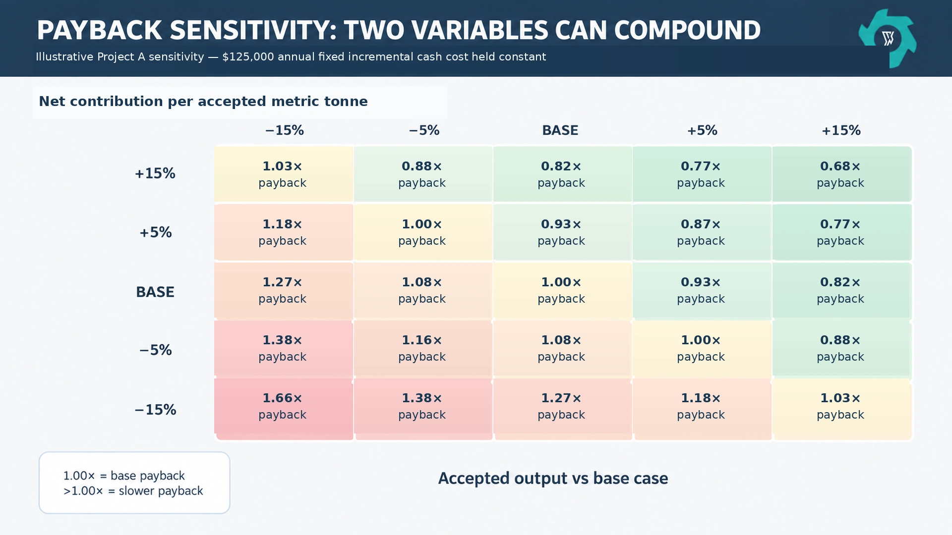
The financial model should not end when the purchase order is signed. Each major assumption should have an evidence source. Factory testing can challenge feed rate, output definition, mass balance and intervention frequency. Site acceptance can test the installed material path with real utilities, downstream equipment and operating staff. The first 30, 60 and 90 days can then replace assumptions with operating averages.
For payback, the most valuable acceptance records are simple: accepted input mass, accepted output mass, the separate reject streams, running time, elapsed time, stops, reversals, operator interventions, manual clearing, downstream holds and maintenance stops. These are not accounting details. They explain why the daily accepted-output number is above or below the investment case.
Do not rewrite the financial model to preserve the original payback promise. Update the model to match evidence. If the line produces less accepted output but also uses less labor than expected, change both inputs. If a reject stream has more saleable metal value than assumed, add the verified credit. If a new customer pays more but requires tighter quality and lower yield, model both effects. An ROI model is useful only while the physical and commercial assumptions remain visible.
Use a Sensitivity Table Before Negotiating the Last 5% of Price
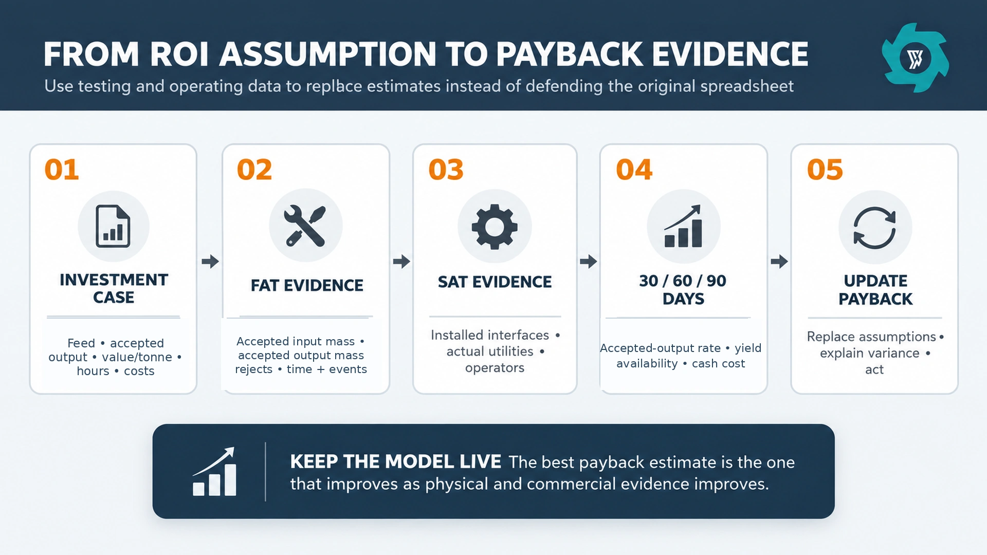
Equipment buyers naturally negotiate purchase price. That matters, but a sensitivity table can show whether the negotiation is focused on the largest value lever. If a 5% price reduction saves $60,000 but a 0.2 t/h improvement in accepted output creates $40,000–$60,000 of annual contribution, the performance assumption may deserve at least as much attention as the discount.
Run the sensitivity one variable at a time first, then combine realistic downside pairs. Accepted output and net contribution often interact. Yield and product quality interact. Uptime and labor overtime interact. A model that only tests each variable independently can still miss the compound case in which difficult feed reduces rate, increases rejects and adds manual work at the same time.
Common ROI Errors That Make Payback Look Better Than It Is
- Using inbound tonnes as product tonnes. Incoming bale mass can include moisture, contaminants and material that becomes reject.
- Using one machine’s capacity as the line capacity. The complete process and downstream state decide accepted output.
- Assuming 100% of scheduled time is productive. Planned maintenance, cleaning, feed changes and downstream holds consume real hours.
- Valuing every paper-bearing reject as product. A stream has value only when there is a defined buyer or use and it meets that acceptance condition.
- Ignoring ramp-up. Cash recovery starts with real commissioning performance, not with the steady-state line in the spreadsheet.
- Using wage rate instead of employer labor cost. Benefits, overtime and staffing coverage can materially change the labor line.
- Forgetting working capital. Inventory and receivables can increase peak cash invested after equipment is installed.
- Keeping one fixed OCC price for the whole study period. Use scenario values or contract-backed assumptions and keep freight and deductions visible.
- Counting tax or financing benefits twice. Keep the operating model and finance model reconciled so the same benefit is not added in two places.
- Freezing the original business case after startup. Replace assumptions with measured operating data and explain deviations.
What a Buyer Should Have Before Calling the ROI “Defensible”
A defensible payback case does not need perfect forecasts. It needs traceable assumptions. Management should be able to see the total cash invested, the accepted-output definition, the production calendar, the assumed ramp curve, the net value per accepted ton, the fixed and variable cash costs, the working-capital requirement and the evidence behind each number.
The model should also show what is intentionally excluded. Tax depreciation, debt service, grants, incentives, salvage value and corporate hurdle rates belong in the final finance model when relevant. Keeping them separate at first helps the engineering team prove the operating case without mixing technical performance with company-specific financing choices.
Finally, connect the model back to the quotation. A supplier does not control OCC market prices, customer payment terms or the owner’s labor agreement. A supplier can, however, define the proposed equipment boundary, accepted feed envelope, test method, expected operating behavior, maintenance access and evidence package. The buyer should assign each ROI variable to the party that can actually verify or manage it.
Plan Your OCC Plant Payback
Share your feed details, target output and operating schedule. YUXI can help define the line and test data for your payback model.
OCC Recycling Plant ROI FAQ
What is a realistic way to calculate OCC recycling plant payback?
Start with total cash invested and model the plant month by month using accepted output, net contribution per accepted metric tonne, fixed incremental cash costs, ramp-up and planned downtime. Simple payback is the point at which cumulative operating cash contribution recovers the initial cash investment. Keep taxes, financing and depreciation in a separate finance model unless they are intentionally part of the decision basis.
Which operating variable has the biggest effect on OCC plant ROI?
There is no universal single driver. In many projects, sustained accepted-output rate during productive running time, accepted yield, operating availability and net contribution per accepted metric tonne interact strongly. A small change in any one may be manageable, but several optimistic assumptions occurring together can move payback by years. That is why sensitivity testing is more useful than one headline payback number.
Should nominal shredder capacity be used in the ROI model?
No. Use sustained accepted output for the complete line under the defined feed and downstream condition. A shredder may reach a high short-term rate while the plant loses time to bale opening, wrapping, downstream holds, reject handling or baler cycles. ROI should follow the tons that meet the accepted-output definition, not the largest nameplate number in the quotation.
How should fiber loss and rejects be treated in the ROI calculation?
Keep accepted input and accepted output weighed separately, together with ferrous output, other rejects, dust or fines, oversize or return material where present, retained material and unexplained difference. Only the stream that meets the commercial accepted-output condition should receive the assumed product value. If a reject has a real by-product value or disposal cost, model that separately rather than hiding it inside an average yield.
When should a buyer use NPV or IRR instead of simple payback?
Use simple payback as a screening measure when management wants to know how quickly invested cash may be recovered. For a final capital decision, a longer-lived project or alternatives with different timing of costs and benefits, add discounted cash-flow measures such as NPV or IRR and a life-cycle cost view. Those methods account for timing and recurring future costs that simple payback does not capture.
References
- AF&PA (2026). Recycling Rates.
- U.S. DOE. Life-Cycle Costs.
- OSHA. Paper Recycling Hazards.
- BLS (June 2026 data). Employer Compensation.
- U.S. EPA (2024). Infrastructure Assessment.